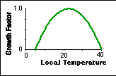
At the beginning of time, the planet is vacant -- no daisies. But the daisies will try to colonize the uncovered land as time goes on and as conditions become favorable for their growth. Each of the daisies has a preferred temperature range; they grow best at an optimum temperature and there are upper and lower temperature limits to the their growth. The model incorporates a growth factor that varies from 1 to 0, defined according the the following equation:

Growth Factor _white = 1-0.003265(22.5-T _white ) ²

The growth factor for the black daisies is calculated in a similar manner. This equation may look complex, but it is just a parabola, as shown in the figure below. This parabola has a peak value of 1 -- the maximum growth factor possible at an optimum temperature of 22.5°C -- and drops to zero at local temperatures of 5°C and 40°C. Thus, growth of the daisies can only occur within this temperature range, but remember that this is the local temperature.

The local temperature of the land around the two types of daisies will differ because of the fact that they absorb different amounts of solar energy. The black daisies absorb more energy and they radiate this energy, heating their surroundings. In contrast, the white daisies reflect more solar energy, which lessens the amount absorbed in that region, so that region ends up being cooler than if there were no white daisies. The local temperature is defined according to the following equation:

T _white = F _HA * (A _planet -A _white ) + T _planet

where A represents the albedo and FHA is the heat absorption factor, initially set at 20.This means that if the albedo of the planet is initially 0.5 and the albedo of the land with white daisies is 0.75, then the local temperature of the white land is 5°C cooler than the average planetary temperature. There is a similar equation for the local temperature of the black land.

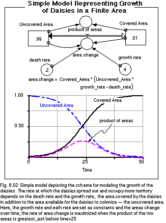
Once the growth factors have been calculated, the model determines how much new area will be gained or lost by each daisy. The way this works is shown in the figure below, a simplified version of the more complex model we'll get to shortly.

In the above figure, note that we use reservoirs to represent the areas. The flow connecting these area reservoirs is a biflow, meaning that area can be transferred in either direction -- the daisies may gain ground by taking it from the uncovered area reservoir, or they may lose ground, in which case area is added to the uncovered reservoir. The question of whether the daisies gain or lose land is a function of the growth factor, the deat rate, andthe area covered and also the area uncovered. In the form of an equation, we can represent this as follows:

area change = area _daisies *(area _un *growth factor - death rate)

This equation basically consists of two parts -- one that gives the area lost because of the natural death rate and one that gives the area gained due to growth of the daisies. The part that determines the area lost because of the natural death rate is pretty simple, but the other part is a bit more complex -- it will tend to be higher when the area covered is higher but also when the area uncovered is higher. The idea here is that with more land covered, there will be more daisies, producing more seeds that can spread out and successfully colonize the remaining land. But as the uncovered land declines, the success rate of seeds also declines because of overcrowding. The complexity here comes from the fact that area reservoirs are connected to each other and their sum at any point in time is equal to a constant value (1 in this case). As can be seen in the above figure, the result is that the rate of area change reaches a maximum when the there is an equal balance between land covered and land uncovered. This model represents a very simple ecosystem, but it is sufficient for the purposes of Daisyworld, which is, after all, a very simple model.

Use the following model diagram and the equations to construct a model of Daisyworld.

10/12